How does something this simple produce something this complex?
Not complicated the way a tax form is complicated, a pile of separate rules stacked on top of each other. Complex the way you could stare at it for years and still not fully explain where it came from, even though the rule behind it fits in one line.
That is what fractals show you, or at least what one specific family of them shows you, since all four fractals below come out from same equation.
$$ z_{n+1} = z_n^2 + c $$
If you have not seen this notation before, don't worry, it's simpler than looks. z and c are just numbers. Pick a value for c, start z at zero, then run equation over and over. Square whatever z currently is, add c to it, and the result becomes the new z. Do it again. And again. Maybe thousand times.
What comes out depends entirely on what question you ask going in, and the four images below are four different questions asked of the exact same line of math.
The Mandelbrot Set
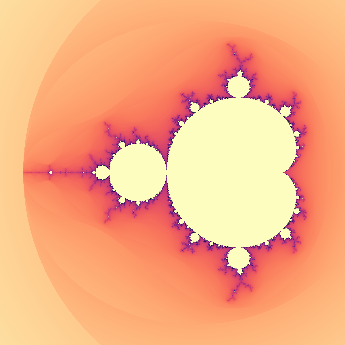
The Mandelbrot set is built around one question. Does z stay small forever, or does it eventually grow without limit?
When you run z = z² + c over and over, one of two things happens. Either z keeps bouncing around near zero, staying manageable no matter how many times you iterate. Or it starts growing, slowly at first sometimes, and once it starts it does not stop, it just gets bigger until it's effectively infinite. That second behavior is what people mean when they say a point escapes.
Which values of c cause z to escape, and which ones don't? For some values it escapes almost immediately, within first five or ten iterations. For others it takes hundreds of iterations before z finally gives up and starts growing. For the values in the black region of the image, z never escapes no matter how long you run it, and those are points that belong to the Mandelbrot set.
The colors outside the black region show how quickly each point escaped, slow escape gets one color, fast escape gets another, that's where all the visual structure comes from and nothing else.
What makes this genuinely strange is the boundary between escapes and doesn't escape. That edge is infinitely detailed. Zoom into any part of it and there is new structure that was not visible at previous scale, spirals containing smaller copies of the whole set, filaments branching into smaller filaments, and it never flattens out no matter how deep you go. Mitsuhiro Shishikura proved in the early 1990s that this boundary has Hausdorff dimension of exactly 2, the highest a shape drawn on flat plane can have, confirming something Mandelbrot himself had conjectured years earlier.
Deep networks build their decision boundaries in loosely similar way. A simple operation, repeated many times through the layers, and the boundary a network learns between yes and no ends up extraordinarily complicated, more complicated than anyone explicitly designed. Nobody sat down and drew that boundary by hand, it came out of the iteration, same way the Mandelbrot set's boundary comes out of one squaring operation, repeated.
Julia Sets
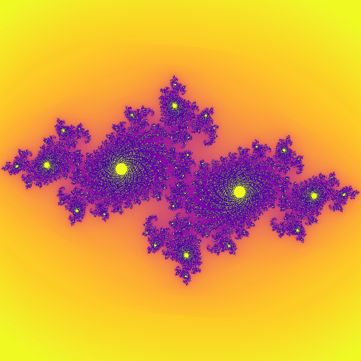
The Julia set uses exact same equation and asks different question.
In the Mandelbrot set, c changes with every pixel and z always starts at zero, so you're really asking, for each value of c, does zero escape or not. The Julia set flips this. c is fixed, one value, locked in, and then you ask which starting values of z stay bounded under that fixed rule.
So instead of testing every possible c, your now testing every possible starting point for z. Same equation, different variable in charge.
Pick c = -0.7269 + 0.1889i and you get the image above. Pick c = -0.4 - 0.6i and the structure looks completely different. Move c by even a tiny amount and fractal can change again, sometimes dramatically.
There is a precise relationship between the two sets. Every point on the Mandelbrot set corresponds to a Julia set shape, so the Mandelbrot is basically a map of every possible Julia set, compressed into one image. Points inside the Mandelbrot produce Julia sets that hold together as one connected piece. Points outside produce Julia sets that shatter into disconnected islands.
This kind of sensitivity to single number shows up in model training too. Change a learning rate slightly, or tweak a regularization term, and a model can end up behaving in totally different way, not just a bit better or worse. The Julia set is a decent way to make that concrete, a tiny shift in c and your looking at a different picture entirely.
Adversarial examples are the sharper version of this. These are inputs changed by tiny, often invisible amounts that cause a model to make a confidently wrong prediction. One of the most influential explanations since Ian Goodfellow's 2014 paper on the subject isn't that networks have some kind of chaotic, fractal shaped decision surface, though that idea does show up in some later papers too. It's closer to the opposite problem, networks built from common activation functions like ReLU end up behaving close to linear across large stretches of very high dimensional input space, and in enough dimensions, small, carefully aimed nudge spread across every input pixel adds up to a large shift in the output. The Julia set is still a fair way to picture the general idea, that tiny input changes can cause huge output changes, it just is not the actual mechanism agreed on for this specific case.
The Burning Ship
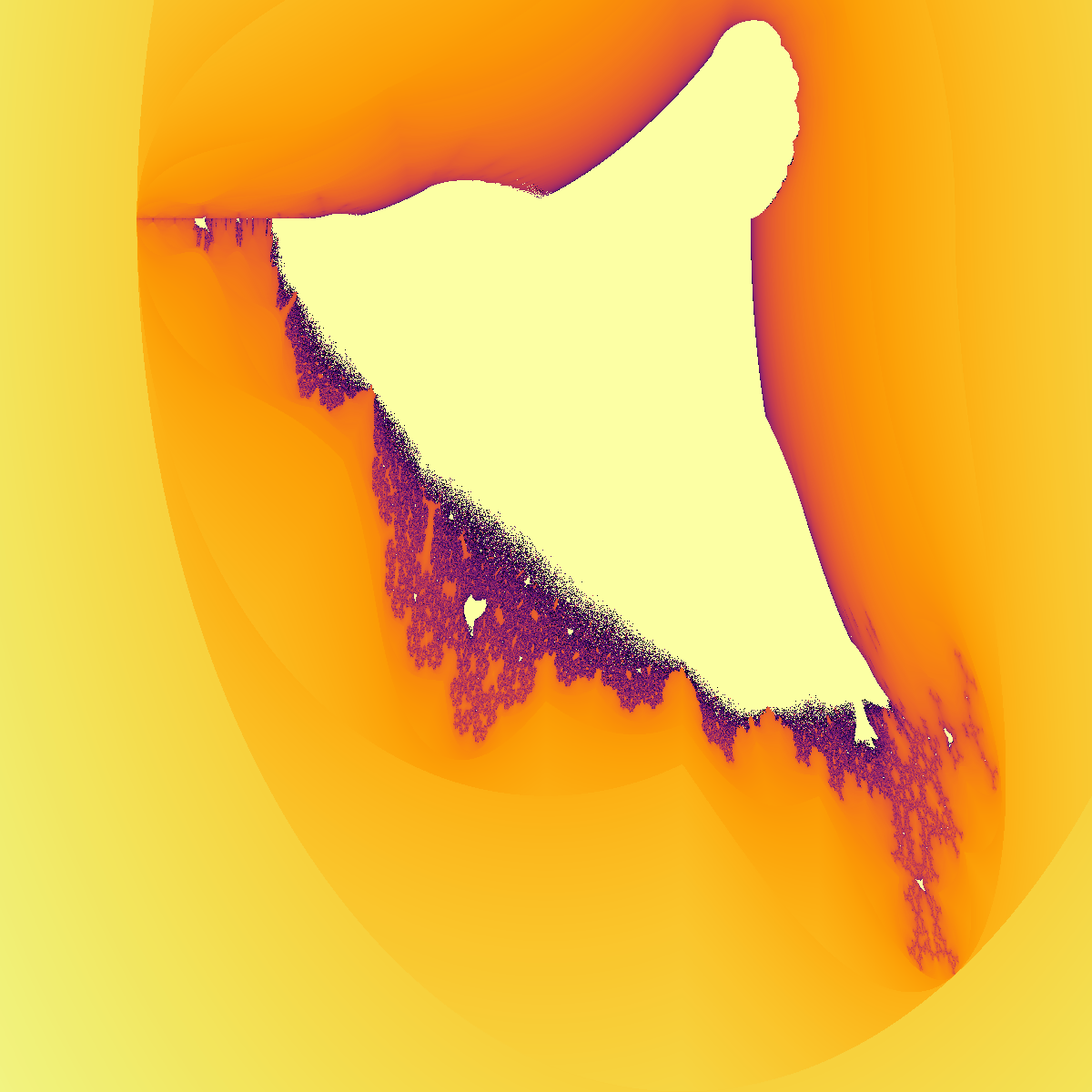
This one is less well known and worth paying attention to. Otto Rössler, a chaos theorist, and Michael Michelitsch first described it in 1992, in short paper called "The Burning Ship and its Quasi-Julia Sets."
The Burning Ship changes exactly one thing about the Mandelbrot iteration. Before squaring z, it forces both of its components to be positive.
$$ z_{n+1} = \left( |\text{Re}(z_n)| + i|\text{Im}(z_n)| \right)^2 + c $$
Quick note on notation, these numbers have two parts, real part and imaginary part, that's the i. Re(z) means the real part of z and Im(z) means the imaginary part. The vertical bars mean absolute value, make whatever is inside them positive. That's entire modification.
One absolute value, applied to each component before squaring, and result shares almost no visual DNA with the Mandelbrot set. The symmetry is gone. In its place is something that looks like ship on fire, with identifiable masts and a hull sitting in lower half of the plane, which is how it got its name.
That modification is smaller than any tweak you'd make training a model, and it changes everything about the output. Architectural decisions in neural networks work the same way, they are not just settings to tune, they are structural changes to the computation itself. Residual connections in ResNets, self attention in transformers, gating in LSTMs, each is structural change to the basic iteration, and each unlocks capability the previous structure did not have. The Burning Ship is a good thing to remember whenever someone argues two architectures are basically same thing. Sometimes one change really does change everything.
The Buddhabrot
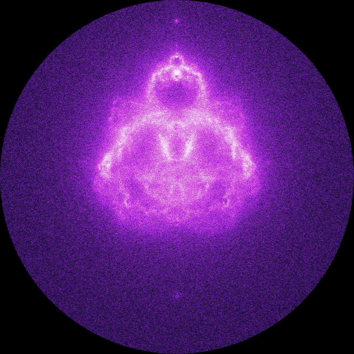
The Buddhabrot does not ask whether a point escapes, it asks where the point went before it escaped. Melinda Green found this technique in 1993 and described it in a post to the sci.fractals newsgroup.
The process works like this. Sample millions of random starting points for c. Throw away any that never escape, since those belong to the Mandelbrot interior and their paths are not useful here. For every point that does escape, record entire path z took during all its iterations before escaping. Pile all of those paths from all of those millions of points on top of each other into single density map. Regions that many orbits passed through on their way to escaping get bright. Regions orbits rarely visit stay dark.
At high enough resolution the result looks like seated, meditating figure. That isn't coded into the math anywhere, it shows up purely because of where these particular orbits happen to travel in the complex plane. It's not even Green's own name for it, either. She first called shape Ganesh, after a colleague recognized the trunk and ears of the elephant headed Hindu god Ganesha in it. The name Buddhabrot came later, coined by Lori Gardi. Color different escape time ranges differently instead of just one density map and you get a variant called the Nebulabrot, which looks a lot more like cosmic cloud than a meditating figure. The equation itself has no opinion on any of this.
Attention maps in transformer models work on similar principle. A transformer doesn't just record the final output for each word, it records which other words each word paid attention to while being processed. Visualize where attention consistently flows across millions of examples and you get something like a learned Buddhabrot, a density map of what the model found worth routing through, not just what it output at the end.
There's also a connection to how diffusion models generate images. The final image is not drawn directly from the model's weights, it emerges from a denoising process applied step by step, dozens or hundreds of times. The image lives in the process, not in any single output, and Buddhabrot works the same way. What you see is the side effect of millions of orbits, nothing was ever explicitly drawn or specified anywhere.
The Perlin Landscape
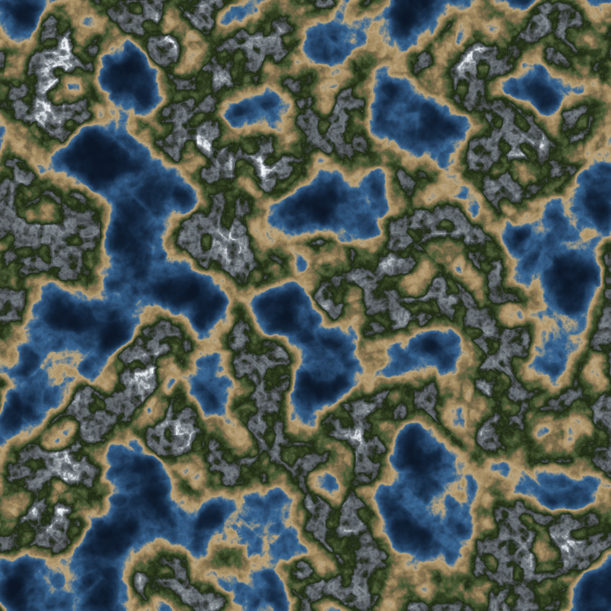
The fractals above are all deterministic, put in the same numbers and you get exact same shape every time. Fractal noise introduces randomness into the equation, but in strictly controlled, hierarchical way.
The foundation is Perlin noise, which Ken Perlin built in 1983 while working on the visual effects for Tron, frustrated with how machine made the computer graphics of that era looked. He described the technique properly two years later, in a 1985 SIGGRAPH paper called "An Image Synthesizer," and eventually won a Technical Achievement Academy Award for it in 1997.
A single layer of Perlin noise doesn't look like much on its own, just a blurry, cloudy grayscale image. Something interesting happens once you layer it using technique called fractal Brownian motion, fBm for short.
Take your base noise, which creates large, smooth, rolling hills. Add second layer, zoomed out so its details are smaller, and reduce its impact, its amplitude. That adds boulders. Add a third layer, smaller still, for rocks, then a fourth for pebbles. Written out, layering looks like this.
$$ f(x) = \sum_{i=0}^{n-1} a^i , \text{noise}(b^i x) $$
Here a is the persistence, how much each smaller layer matters, and b is the lacunarity, how fast frequency increases each time.
Open world video games are real world instance of this equation at work, generating heightmaps too large to hand sculpt one hill at a time. Low frequency noise lays down the mountain ranges and plains, and each higher frequency layer on top adds finer terrain detail, roughly the way f(x) describes.
Some image generating models build pictures same coarse to fine way. StyleGAN, built for generating realistic faces, adds randomness at several stages while building an image, early stages set the big things like the general shape of the face, later stages add the small stuff, individual hair strands and skin texture. Rough shape first, fine detail stacked on after, same idea as the terrain.
Diffusion models, the kind behind most AI image generators, often do something similar, they build small rough version of the image first, then sharpen it in passes. This pattern shows up even where nobody designed it that way on purpose, too. A network trained just to recognize what's in a photo tends to organize itself the same way on its own, early layers pick up big basic shapes and colors, deeper layers pick up fine texture and edges. Nobody tells it to work like that, it's just the easiest way to make sense of a picture, same reason Perlin reached for it in 1983.
The Part That Is Actually Useful
Beyond the visuals, fractal geometry gives concrete way to measure how rough or irregular a signal is. The idea is called fractal dimension. A perfectly smooth curve has a dimension of 1, a flat plane has a dimension of 2, and the Mandelbrot boundary we just saw sits at true maximum of 2. Real world signals usually sit somewhere between those extremes.
This matters for a few practical things.
Anomaly detection. Systems behaving normally tend to have consistent fractal properties over time, and there's a real body of research using this, mostly around network traffic. Internet traffic is famously self similar across timescales, and when that fractal structure shifts, it can be sign of a DDoS attack or other unusual activity before anything else flags it. Same general idea gets applied to industrial sensors, where a shift in the fractal dimension of a reading can catch equipment wear early.
Time series features. Fractal dimension, especially something called Higuchi method, is a real feature used for classifying signals like EEG and heart rate variability, sometimes to tell emotional states or brain activity apart in ways plainer statistics on the same signal do not capture as well.
Checking generative models. There's growing interest in using fractal metrics to check whether images or text produced by generative model carry the same statistical self similarity as real data. A model can score well on standard evaluation metrics while still missing something structural about the distribution it was trained on, and fractal dimension is one way to go looking for that gap.
The Part Worth Sitting With
Large language models and deep networks keep surprising the people who build them. Capabilities appear that were not explicitly trained for. Internal structure forms that nobody designed. There's a lot of mysticism attached to this, but the fractal parallel makes it feel less mysterious, if not less impressive.
The Mandelbrot set does not have its shape because someone drew it that way. The shape exists because iteration dynamics of z = z² + c produce a region of stability whose boundary happens to look like that. The structure is a consequence of the rule, nobody planned it, and nobody could have predicted its exact outline just by staring at the rule on paper.
Neural networks work in similar way. The rule is, minimize this loss, adjust these weights, repeat. What emerges from doing that millions of times on large dataset isn't something you can predict from the rule alone. The structure is real, the rule behind it is simple, and gap between the two is roughly where interpretability research lives.
The honest position is that this structure gets studied the same way mathematicians study fractals, by running the process many times and looking carefully at what accumulates. Nobody derives the Buddhabrot with pen and paper, you simulate it and observe. Mechanistic interpretability is not doing something identical to that, the math underneath is completely different, but basic posture is same, run the system across many inputs and watch closely for which parts activate, which features form, which paths consistently matter.
The equation is short. What it produces is not.
The Code
All four fractals live in single R file with consistent output settings, 1200x1200 pixels, black background, no margins, and perceptually uniform color palettes from the viridis package. The Mandelbrot, Julia, and Burning Ship use vectorized matrix operations in pure R. The Buddhabrot uses C++ through Rcpp with parallel workers, since tracking millions of orbits at 1,500 iterations each isn't something R handles gracefully on its own.
Source: mandelbrot_family.R
I keep coming back to how short that one line of math is compared to everything it's able to produce, and how much of modern machine learning ends up rediscovering same lesson at much bigger scale. If any of the ML comparisons above are stretched too far or just plain wrong, email me, I'm learning most of this alongside writing it down.